Was there a bubble for Remain on the night of the EU referendum?

by Tom Auld, CERF Research Associate, Cambridge Judge Business School, University of Cambridge

The UK’s vote for Brexit on 23 June 2016 was the first great political shock of that year (the second being Donald Trump’s win in the US presidential election). It had profound effects on financial markets (Aristeidis and Elias, 2018; Alkhatib and Harasheh, 2018; Sultonov and Jehan, 2018; Caporale et al., 2018). Global risk assets sold off sharply, with the pound immediately losing over 10% against the dollar. The result was also seemingly against all expectations. Betting odds for leaving the EU were around 4 to 1 during the final week of the campaign and bottomed out at 10 to 1 shortly after voting closed. This was despite tight polling that showed only a small lead for remain within the margin of error of most polls. Much of the literature on the topic suggests the possibility of the presence of mass bias in beliefs about the UK’s voting intentions, with a bubble in opinion for remain (Gelman and Rothschild, 2016; Fry and Brint, 2017; Wu et al., 2017). But the question remains, did this bias for remain persist on the night of the EU referendum as results were announced?

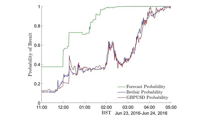
Figure 1: Probability of Brexit chart

How the night unfolded

The night of the referendum provided a unique opportunity to study market efficiency. It is not controversial to assume that the only information relevant to financial asset prices during the night was the referendum. Furthermore, the results from 382 distinct voting districts would be released at different times over the course of a few hours. Information was slowly drip fed to the markets during what is usually a quiet overnight session.

Voting closed at 10pm. Two minutes later YouGov released a poll on the day. This showed a small lead of 51.6% for remain versus 48.4% for leave. The sampling standard error was 3%. This implies the lead for remain was well within the margin of sampling error (let alone the systematic error in polling methodology). At the same time, the betting markets were implying around a 10% likelihood of Brexit.

Around midnight results began to arrive. By 1:17am ten areas had reported. Eight had vote-shares for Brexit above expectation. The average shock in these first results was +3.2% for Brexit. If repeated nationally this swing would reverse the lead for remain. Risk assets began to sell off as the results arrived, but the descent took until well after 4am for the electorate’s decision to be fully reflected. The BBC finally projected a vote to leave the EU at 4:39:32am.

A novel Bayesian approach

Previous work (Wu et al., 2017) attempted to demonstrate market inefficiency in the pound market using an asymptotic OLS based electoral modelling approach. However, such an approach relies on large numbers of results being known to accurately model the distribution of the unknown vote for Brexit. However, by the time sufficient datapoints are available it can be argued (and we do) that the result should already be known.

A method is required that enables an analyst to make a forecast knowing only few results (or one, or even zero!) We achieve this using a novel Bayesian methodology. The Bayesian approach uses a prior probability distribution that encapsulates beliefs about the likelihood of the unknown result. Those beliefs are updated as information becomes known via Bayes rules. Our prior is a joint semi-parametric distribution of the results of all 382 voting districts. We make use of expectations for these areas published by psephologist Chris Hanretty on 7 June 2016 in a blog titled ‘What to expect on the night.’ These are used to calibrate our prior. Following updates in real-time as results arrive, an implied probability for Brexit is simulated. We also calculate implied probabilities of Brexit from financial asset prices, making use of the fact that financial prices are cointegrated with betting markets under certain conditions (Auld, 2022). We can then relate our electoral model probabilities to those implied by the real time evolution of the market determined prices. We find that both betting and financial markets appear to be slow in absorbing the information contained in the vote by around 3 hours.

A fully robust conclusion

Our model relies on the choice of several hyperparameters to represent investor beliefs at the start of the night through the prior distribution. One could of course object to any of the values chosen. As part of robustness check we vary hyperparameters and check our results. We find that only 2 variables meaningfully affect the speed of converge.

The first hyperparameter of interest is the level of uncertainty in our prior. This is represented by the standard error in the vote share for Brexit. It is equivalent to the prior belief of the systematic error of recent polls. We find a standard error for general elections in polling error of around 2.5%. The higher the standard error, the higher the starting probability for Brexit but the slower the convergence to certainty. It is inconceivable that the once in a lifetime Brexit referendum could have polls as accurate as general elections (which occur every 4 years). We chose a conservative value of 5% in our core model. However, we find that increasing this hyperparameter does not change our conclusions meaningfully.

The second hyperparameter that is important is the correlation ρ between shocks from different constituencies. The higher the value of ρ the greater the effect a surprise in one area will have on the expectations of those in others yet to announce. Thus, higher ρ will cause faster convergence. For general elections this value is around 0.3. However, we again find that varying ρ below 0.3 significantly does not change our core conclusion that markets were slow to price Brexit by the order of hours.

Simply irrational behaviour

The Bayesian approach allows us to go one step further in our analysis and ask what possible values of hyperparameters in our prior, and hence investor beliefs, are implied by market behaviour. We find that the markets were so slow to reflect the results that a value for ρ of between zero and 0.01 is required. This is close to assuming shocks from the one voting district are fully independent of others. It can be shown that ρ is the ratio of systematic national polling error variance to total variance of all constituency polling errors. For general elections this ratio is found to be stable and around 30%. It is unthinkable that investors could believe that only 1% of the variance of the collection of the 382 results is explained by the national polling error. It is as though investors failed to price in any effect of the surprises for Brexit from the initial results on the large numbers of areas yet to report. The conclusion is that both bettors and investors in financial markets were simply irrational and could not believe that the UK was voting to leave the UK.

The conclusion of this work is that without a shadow of a doubt the bubble for remain persisted well into election night.

This blog is based upon published work co-authored with Professor Oliver Linton, current Chair of the Faculty of Economics.